Introduction
There are certain movies (could be anything) that some people like, and certain movies that they don't. Based on their movie ratings, a recommender system can be implemented to suggest other movies that they may like.
To demonstrate this, I will use the dataset from [MovieLens](https://grouplens.org/datasets/movielens/), where users have rated on some movies.
import pandas as pd
from collections import defaultdict
import numpy as np
import matplotlib.pyplot as plt
Data Analysis
Let's see the first few elements of the data. There are 4 columns: userId, movieId, rating, and timestamp.
df_ratings = pd.read_csv('ml-latest-small/ratings.csv')
df_ratings.head()
Let's merge movie titles and genres into the data frame.
df_movie = pd.read_csv('ml-latest-small/movies.csv')
df = pd.merge(df_movie,df_ratings)
df.head()
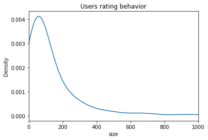
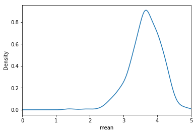
Let's inspect the patern of how the users rated the movies.
df.groupby('userId').agg({'rating':[np.size,np.mean]}).describe()
There are 671 users. On average, a user rated 149 movies. The average rating given by a user is around 3.7.
df.groupby('userId').agg({'rating':[np.size,np.mean]})['rating']['size'].plot.density()
plt.title('Users rating behavior')
plt.xlim(0,1000)
plt.xlabel('size')
plt.show()
df.groupby('userId').agg({'rating':[np.size,np.mean]})['rating']['mean'].plot.density()
plt.xlim(0,5)
plt.xlabel('mean')
plt.show()
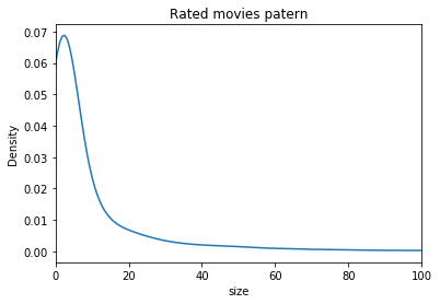
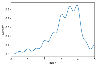
Let's inspect the patern of how the movies are rated.
df.movieId.value_counts()[:10]
df.groupby('movieId').agg({'rating':[np.size,np.mean]}).describe()
There are 9066 movies being rated. The average number of ratings and the average rating received for each movie is 11 and 3.3. More than 75% of the movies have less than 10 number of ratings.
df.groupby('movieId').agg({'rating':[np.size,np.mean]})['rating']['size'].plot.density()
plt.title('Rated movies patern')
plt.xlim(0,100)
plt.xlabel('size')
plt.show()
df.groupby('movieId').agg({'rating':[np.size,np.mean]})['rating']['mean'].plot.density()
plt.xlim(0,5)
plt.xlabel('mean')
plt.show()
Let's find the most popular movies!
df.groupby('title').agg({'rating':[np.size,np.mean]}).sort_values([('rating','mean')],ascending=False)[:5]
These movies have 5/5 rating, but only has one number of rating, which does not represent the popularity of the movies.
Let's only consider movies with at least 100 number of ratings.</font>
at_least = df.groupby('title').agg({'rating':[np.size,np.mean]})['rating']['size'] >= 100
df.groupby('title').agg({'rating':[np.size,np.mean]})[at_least].sort_values([('rating','mean')],ascending=False)[:5]
Here's the top 5 most popular movies with at least 100 number of ratings. The highest (mean) rating is 4.5.
Collaborative Filtering Recommender System
After the data analysis, let's implement some recommendation systems.
There are primarily two types of recommender systems, i.e. collaborative filtering (CF) and content-based recommation.
CF adopts users attitutes towards the items, while content-based recommender focuses on the item's attributes and make suggestions based on item similarities.
We will focus on CF. There are a few models associated with CF, and I'll compare using k-Nearest Neighbours (kNN) and matrix factorization.
kNN looks for clusters of similar users based on common ratings and make predictions using the average rating of top k-th nearest neighbours. On the other hand, matrix factorizarion find the interactions between users and items by decomposing large matrices, hence make this method more powerful.
Let's do this in the Surprise framework.
from surprise import SVD, Dataset, Reader, KNNBasic, accuracy
from surprise.model_selection import cross_validate
reader = Reader(rating_scale=(1,5))
data = Dataset.load_from_df(df[['userId','movieId','rating']], reader=reader)
k-Nearest Neighbours
Let's start with kNN using cosine similarity.
algo_kNN = KNNBasic(sim_options = {'name':'cosine', 'user_based': False})
cross_validate(algo_kNN, data, measures=['RMSE','MAE'], cv = 5, verbose = True)
RMSE and MAE of 5-fold CV using kNN are 1.0 and 0.8.
Matrix Factorization (Single Value Decomposition)
Let's switch to matrix factorization. One model is the single value decomposition (SVD).
algo_SVD = SVD()
cross_validate(algo_SVD, data, measures=['RMSE','MAE'], cv = 5, verbose = True)
RMSE and MAE of 5-fold CV using SVD are 0.9 and 0.7, which is slightly better than kNN as expected.
From our previous data analysis, a user on average rated 149 movies. Since there are about 160k movies in the dataset, so most of the movies are not rated by the users, in other words, the user-by-item matrix is pretty empty. So we can use SVD to predict the ratings for the other movies that a user has not seen, and output the few movies with highest ratings, hence the birth of our recommendation system.
trainset = data.build_full_trainset()
testset = trainset.build_anti_testset()
algo = SVD()
algo.fit(trainset)
prediction = algo.test(testset)
prediction[:3]
accuracy.rmse(prediction, verbose=True)
n = 10
top_n = defaultdict(list) # Create a pseudo list
for uid, iid, r_ui, est, _ in prediction:
    top_n[uid].append((iid,est))
for uid, user_ratings in top_n.items():
    user_ratings.sort(key=lambda x: x[1], reverse = True)
    top_n[uid] = user_ratings[:n]
for uid, user_ratings in top_n.items():
    if uid == 1:
        #print(uid, [iid for (iid, _) in user_ratings])
        [print(df_movie.query('movieId=='+str(i)).title.values) for i in [iid for (iid, _) in user_ratings]]
These are the top 10 movies recommended for user 1.


